
| 일 | 월 | 화 | 수 | 목 | 금 | 토 |
|---|---|---|---|---|---|---|
| 1 | 2 | 3 | 4 | |||
| 5 | 6 | 7 | 8 | 9 | 10 | 11 |
| 12 | 13 | 14 | 15 | 16 | 17 | 18 |
| 19 | 20 | 21 | 22 | 23 | 24 | 25 |
| 26 | 27 | 28 | 29 | 30 | 31 |
- 데이터불균형
- 파이썬
- 언더샘플링
- 텍스트분석
- dataframe
- 데이터분석전문가
- iloc
- LDA
- opencv
- PCA
- 크롤링
- t-test
- 워드클라우드
- pandas
- 주성분분석
- ADP
- 독립표본
- 데이터분석
- Python
- DBSCAN
- 빅데이터
- 오버샘플링
- Lambda
- 빅데이터분석기사
- ADsP
- numpy
- 군집화
- datascience
- 데이터분석준전문가
- 대응표본
Data Science LAB
[Python] ADP 실기 대비 기출문제 (15회) 본문
문제 링크 : https://www.kaggle.com/code/kukuroo3/problem4-python/notebook
problem4-python
Explore and run machine learning code with Kaggle Notebooks | Using data from ADP_KR_p4
www.kaggle.com
1번
철강데이터 종속변수 : target
데이터 출처 : https://www.kaggle.com/uciml/faulty-steel-plates
데이터 경로 : /kaggle/input/adp-kr-p4/problem1.csv
1-1 EDA(탐색적 데이터 분석)을 하시오
(시각화와 통계량을 제시할 것)
df1 = pd.read_csv('/kaggle/input/adp-kr-p4/problem1.csv')
df1.head()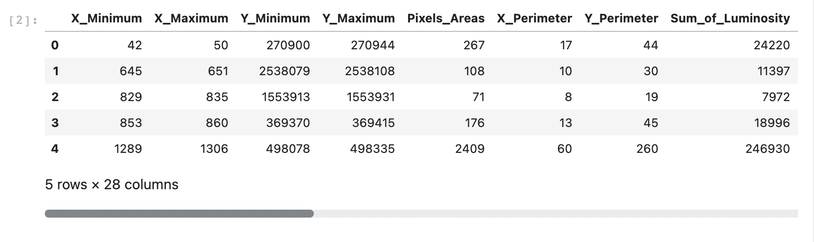
df1.info()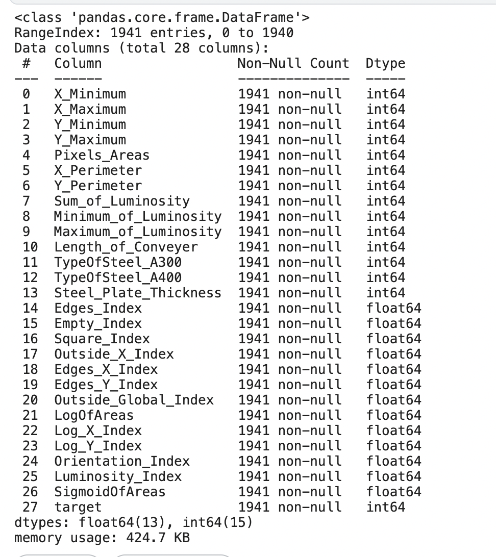
모든 변수가 수치형 변수로 구성되어 있는 것을 확인
df1.describe()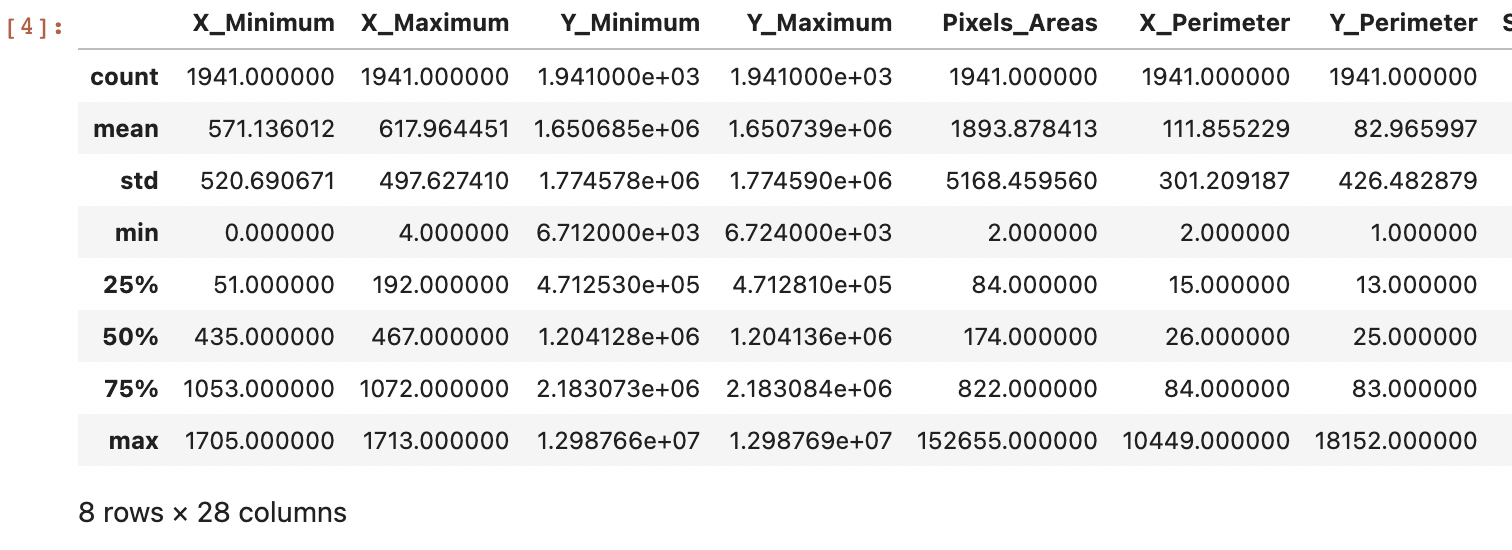
수치형 변수의 데이터 분포 형태를 확인 -> X_Minimum, X_Maximum같은 변수는 평균과 max값의 차이가 크기 때문에 이상치가 존재할 것이라고 예상
df1.isna().sum()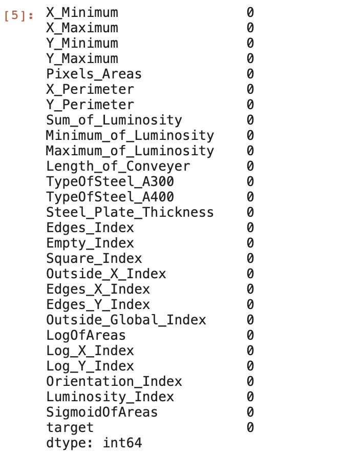
import matplotlib.pyplot as plt
import seaborn as sns

fig, ax = plt.subplots(1,1,figsize=(8,6))
sns.countplot(x='target', data=df1)
plt.show()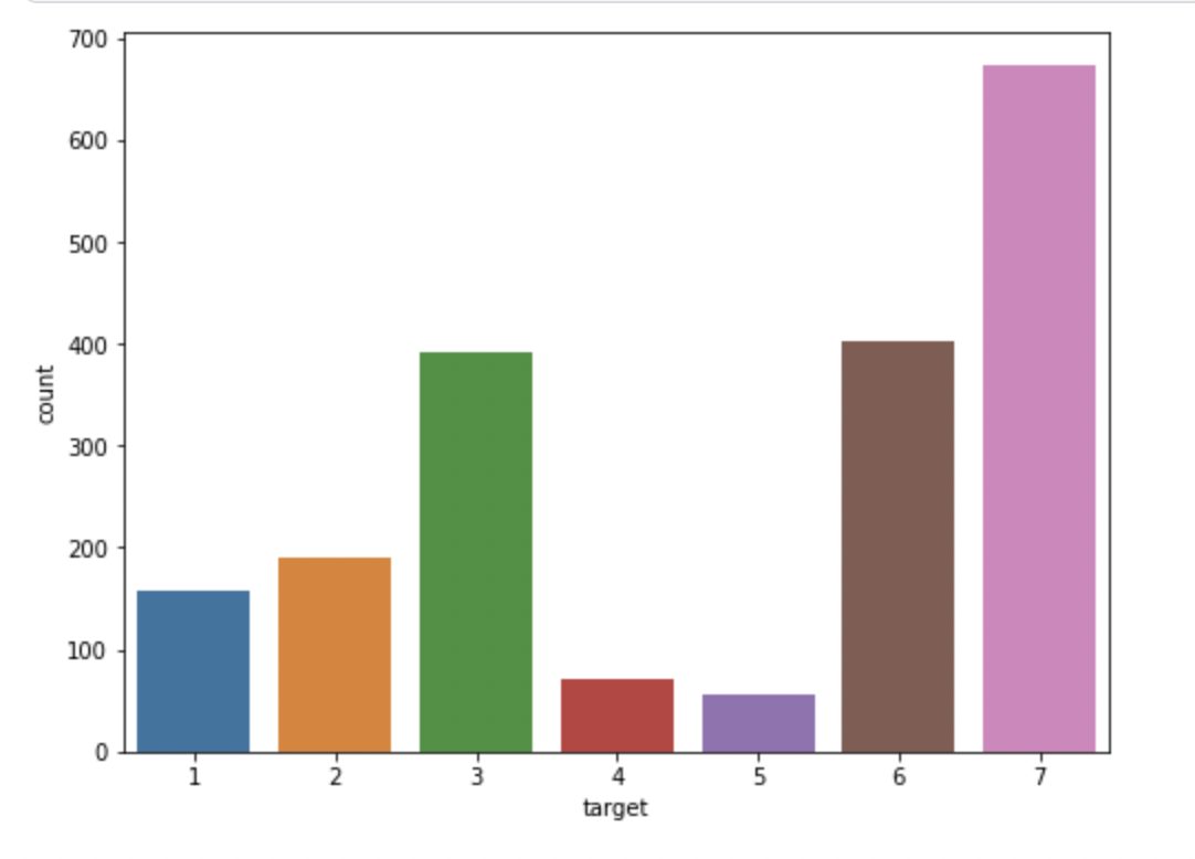
종속변수인 'target'은 1~7사이의 정수로 구성되어 있으며, 그중 7이 가장 많은 것을 확인하였다.
- 회귀분석
- 다중 분류
- 특정한 숫자(ex:1)을 기준으로 0/1로 재구성후 분류 모델 생성
다중 분류 또는 이항 분류가 적절할 것으로판단
df1.plot(kind='box', subplots=True, layout=(4,7), figsize=(20,10))
plt.tight_layout()
plt.show()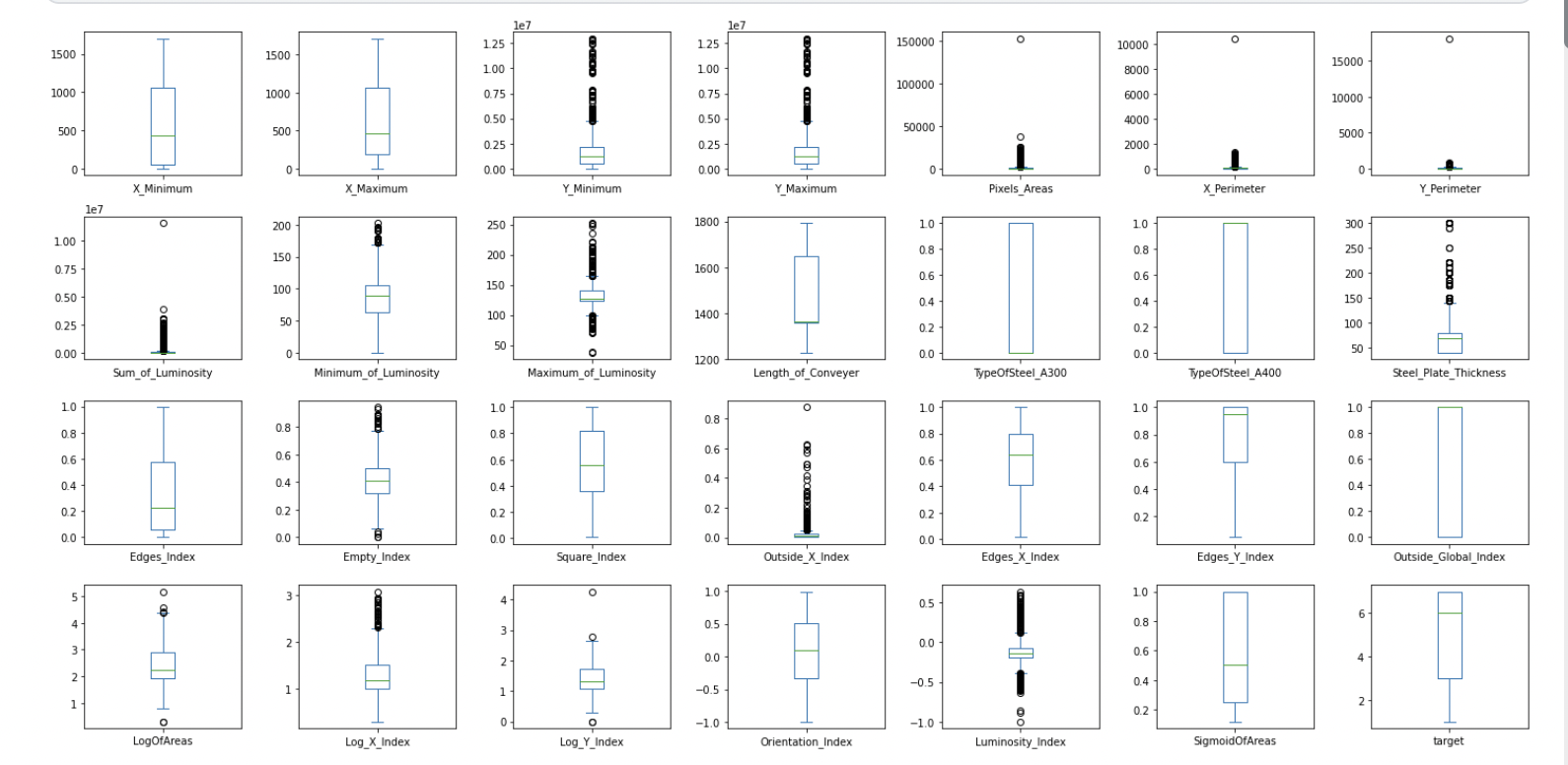
모든 변수에 대체적으로 많은 이상치가 존재하는 것을 확인함 -> 정규화를 통한 스케일 변환이 필요해 보임
1-2 변수 선택(VIF), 파생변수 생성, 데이터 분할(train/test(20%))
(시각화와 통계량을 제시할 것)
from statsmodels.formula.api import ols
from statsmodels.stats.outliers_influence import variance_inflation_factor

df1['av']  = (df1['X_Minimum'] + df1['X_Maximum'])/2
value ='+'.join(list(df1.drop(columns=['target']).columns))
model = ols(f'target ~ {value}', df1)
model.exog_names


vif = pd.DataFrame({'col': col, 'VIF': variance_inflation_factor(model.exog, i)}
             for i, col in enumerate(model.exog_names[1:])).sort_values('VIF',ascending=False)

vif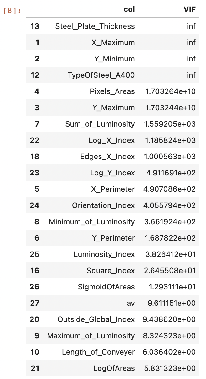
VIF값이 10이상이면 다중공선성이 존재한다고 판단 -> 삭제
10 미만인 변수 : X_Minimum, Edges_Index, Empty_Index, Outside_X_Index, TypeOfSteel_A300, Edges_Y_Index, LogOfAreas, Length_of_Conveyer, Maximum_of_Luminosity, Outside_Global_Index, av
from sklearn.model_selection import train_test_split

X = df2[list(df2.columns.difference(['target']))]
y = df2['target']

X_train, X_test, y_train, y_test = train_test_split(X, y, random_state=0, test_size=0.2, stratify=y)
print(X_train.shape, X_test.shape)
print(y_train.shape, y_test.shape)

# (1552, 11) (389, 11)
# (1552,) (389,)
1-3 종속변수들중 "1"인지 아닌지 판단하려한다. 종속변수를 1과 1이 아닌 값(이항)으로 치환하고 로지스틱 회귀 분석을 실시하라.
confusionMatrix를 확인하고 최적의 cut off value 정하여라.
X2 = X.copy()
y2 = y.apply(lambda x: 1 if x==1 else 0)
print(y2.value_counts())

X_train2, X_test2, y_train2, y_test2 = train_test_split(X2, y2, test_size=0.2, stratify=y2, random_state=0)
print(X_train2.shape, X_test2.shape)
print(y_train2.shape, y_test2.shape)

# 0    1783
# 1     158

# (1552, 11) (389, 11)
# (1552,) (389,)
y_train2.value_counts()

# 0    1426
# 1     126
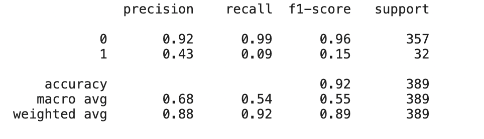
0과 1이 고르게 분포되어 있지 않음
from sklearn.linear_model import LogisticRegression
from sklearn.metrics import confusion_matrix

lr = LogisticRegression(solver = 'liblinear')
lr.fit(X_train2, y_train2)

lr_pred = lr.predict(X_test2)
proba = lr.predict_proba(X_test2)


from sklearn.metrics import classification_report, roc_curve

print(classification_report(y_test2, lr_pred))
from sklearn.metrics import plot_roc_curve

fpr, tpr, threshold = roc_curve(y_test2, proba[:,1])

# get the best threshold
J = tpr - fpr
ix = np.argmax(J)
best_threshold = threshold[ix]

print('Best Treshold = %f, sensitivity = %.3f, specificity = %.3f, J = %.3f' %(best_threshold, tpr[ix], 1-fpr[ix], J[ix]))

# Best Treshold = 0.128821, sensitivity = 0.938, specificity = 0.838, J = 0.775
from sklearn.metrics import roc_auc_score

# plot roc and best threshold
sens, spec = tpr[ix], 1-fpr[ix]

#plot the roc curve for the model
plt.plot([0,1], [0,1], linestyle='--', markersize=0.01, color='black')
plt.plot(fpr, tpr, marker='.', color='black', markersize=0.05, label='auc = %.3f' % roc_auc_score(y_test2, proba[:,1]))
plt.scatter(fpr[ix], tpr[ix], marker='+', s=100, color='r',
           label = "Best Threshold = %.3f"%(best_threshold))

plt.xlabel('False Positive Rate')
plt.ylabel('True Positive Rate')
plt.legend(loc = 'lower right')

plt.show()
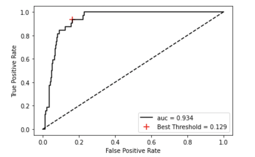
빨간점이 최적의 임곗값
1-4 종속변수(y)를 다항(7 class)인 상태에서 SVM을 포함하여 3가지 알고리즘으로 평가하라.
각 모델에서 confusionMatrix를 확인하고 최적의 cut off value 를 정하여라.
from sklearn.svm import SVC
from sklearn.ensemble import RandomForestClassifier
from sklearn.tree import DecisionTreeClassifier
from sklearn.metrics import accuracy_score,classification_report

svc = SVC(C=0.5)
rf = RandomForestClassifier()
dc = DecisionTreeClassifier()

def cf_mat(model):
    model.fit(X_train, y_train)
    pred = model.predict(X_test)
    print('model : ', model)
    print(classification_report(y_test, pred),'\n')
    print('정확도 : ',accuracy_score(y_test, pred))

    return pred
모델을 훈련시키고 정확도와 classification_report를 출력하는 함수 생성
svc_pred = cf_mat(svc)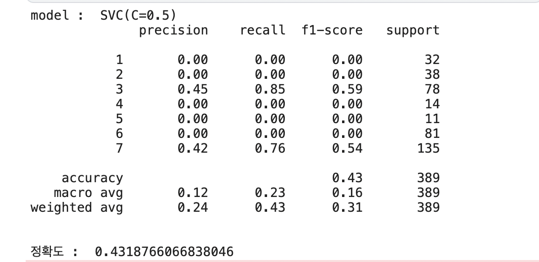
rf_pred = cf_mat(rf)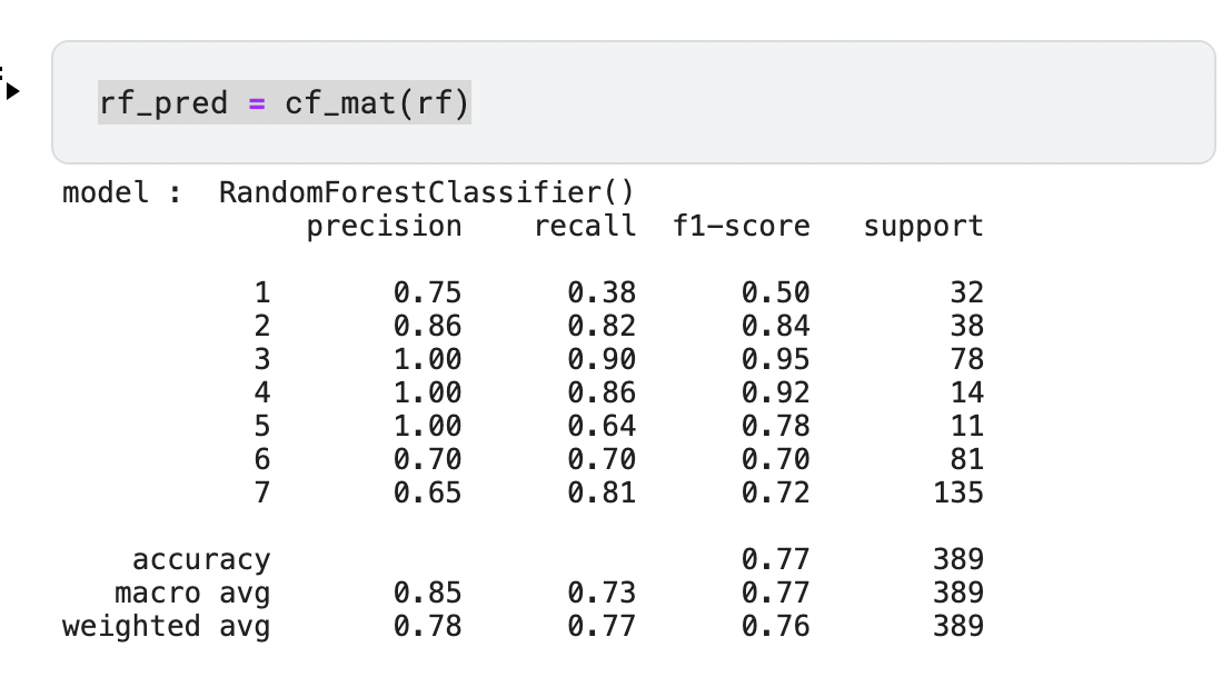
dc_pred = cf_mat(dc)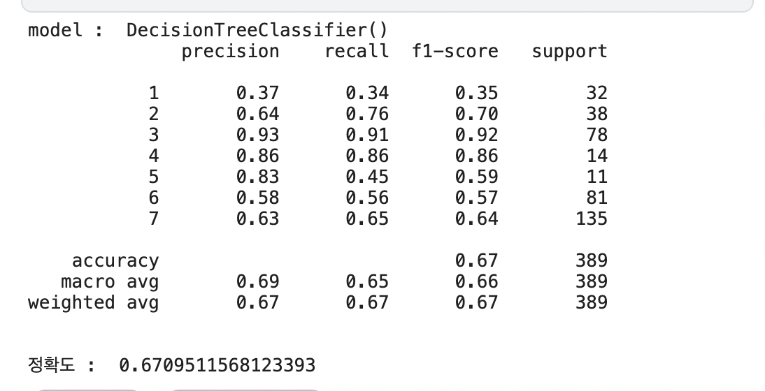
정확도는 RandomForest모델이 0.76으로 가장 높음
정확도 향상을 위해 하이퍼파라미터 튜닝이 필요해 보임
1-5 종속변수를 제외한 나머지 데이터를 바탕으로 군집분석을 실시하고 최적의 군집수와 군집 레이블을 구하여라.
군집레이블을 추가한 데이터를 1-4에서 만든 모델중 가장 성능이 좋았던 하나의 모델에 다시 학습하여 F1-score를 비교하라
from sklearn.cluster import KMeans

def elbow(X):
    sse = []
    for i in range(1,11):
        km = KMeans(n_clusters=i, random_state=0)
        km.fit(X)
        sse.append(km.inertia_)

    plt.plot(range(1,11), sse, marker='o')
    plt.xlabel('The Number of Cluster')
    plt.ylabel('SSE')
    plt.show()
    print(sse)

elbow(X_train)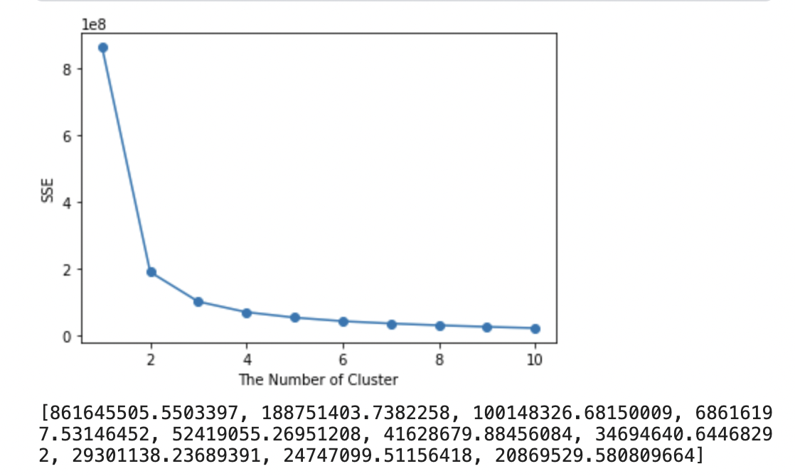
최적의 군집의 개수는 3으로 판단
# 최적의 k로 K-Means 군집화 실행
km = KMeans(n_clusters = 3, random_state=0)
km.fit(X_train)
train_label = km.predict(X_train)
test_label = km.predict(X_test)

X_train_cluster = X_train.reset_index(drop=True).copy()
X_test_cluster = X_test.reset_index(drop=True).copy()

X_train_cluster.loc[:, 'cluster'] = train_label
X_test_cluster.loc[:, 'cluster'] = test_label

rf = RandomForestClassifier()
rf.fit(X_train_cluster, y_train)
rf_pred = rf.predict(X_test_cluster)
print(classification_report(y_test, rf_pred))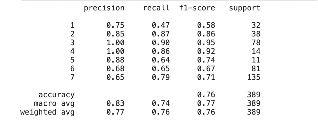
정확도가 가장 높았던 랜덤포레스트 모델에 KMeans를 적용함
f1 score값은 군집 생성 전과 크게 달라지진 않았지만 약간 감소하였다.
2번 전력데이터
데이터 출처 : 직접제작
데이터 설명 : 2050년 1년동안의 5유형(A,B,C,D,E)의 전력사용량을 나타낸다. 각유형의 전력사용량은 1분마다 갱신되며 그 값은 누적된다.
6시간이 지나면(00:00, 06:00, 12:00, 18:00시에) 전력사용량은 0으로 초기화 된다.
- /kaggle/input/adp-kr-p4/problem2_usage.csv
6시간 간격의 총 전력사용량의 데이터이다. timestamp순서는 섞여있다.
6시간 간격의 특정 시간대(마지막시각 '05:59','11:59','17:59','23:59')의 전력 총합을 나타낸다.
데이터의 총합을 구해서 비교할때 부동소수점 오류가 날수 있다. 파이썬의 경우 round(4)를 취하여 해결한다.
- /kaggle/input/adp-kr-p4/problem2_usage_history.csv
1분간격의 A,B,C,D,E 유형의 소비 누적 전력을 나타낸다. 같은 6시간간격의 시간대의 데이터는 같은 "6hour_index"값을 가진다.
00:00, 06:00, 12:00, 18:00시에는 5유형의 전력은 초기화 된다.
데이터의 총합을 구해서 비교할때 부동소수점 오류가 날수 있다. 파이썬의 경우 round(4)를 취하여 해결한다.
- /kaggle/input/adp-kr-p4/problem2_avg_tem.csv
2050년 1년동안 일자별 평균 온도를 나타낸다.
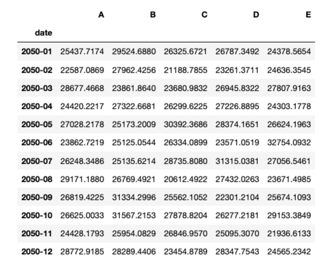
2-1 usage의 총사용량을 아래와 같은 모양으로 연월별 총합으로 계산하여 CSV 파일로 작성하시오.
- 일자별 총사용량은 누적사용량이 갱신되기 직전의 최대값들의 합으로 계산한다
- ['05:59','11:59','17:59','23:59'] 시간대의 A,B,C,D,E의 컬럼별 총합이 각 유형의 일일 사용량이다
us = pd.read_csv('/kaggle/input/adp-kr-p4/problem2_usage.csv')
ush = pd.read_csv('/kaggle/input/adp-kr-p4/problem2_usage_history.csv')

us['time'] = pd.to_datetime(us.timestamp, unit='s')
us = us.sort_values('time').reset_index(drop=True)

s = ush[ush['hh:mm'].isin(['05:59', '11:59', '17:59', '23:59'])]
s2 = s.copy()
s2.loc[:,'t'] = s.iloc[:,2:].sum(axis=1).round(4)


zz = pd.merge(ush, pd.merge(s2.rename(columns = {'t':'usage'}).reset_index(drop=True),us)[['6hour_index','time']])
zz['time'] = pd.to_datetime(zz['time'])

q = zz[zz['hh:mm'].isin(['05:59', '11:59', '17:59', '23:59'])].copy()
q.loc[:,'date'] = q['time'].dt.strftime('%Y-%m')
q.groupby('date').sum()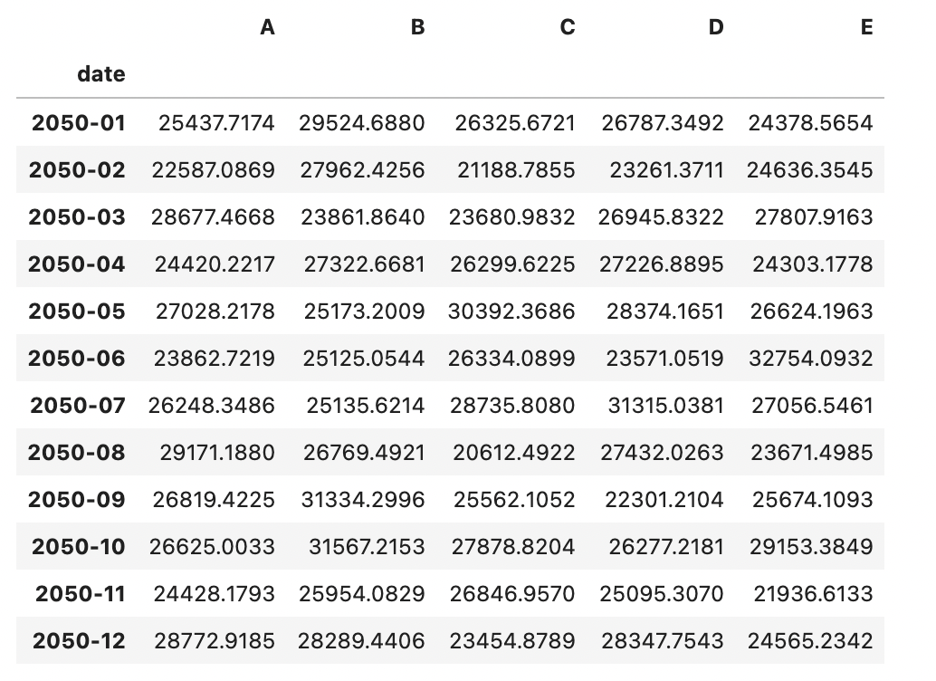
2-2 가로축을 요일(일~월) 세로축을 평균 전력사용량으로 하는 그래프를 그려라. 각 유형별로 색을 다르게 표현하여 5개의 line plot을 그리며 범례를 표시하라
q['day'] = q['time'].dt.day_name()
daydf = q.groupby(['day']).mean().reindex(['Sunday','Monday','Tuesday','Wednesday', 'Thursday','Friday', 'Saturday'])
daydf.plot()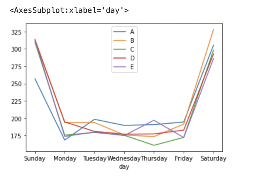
daydf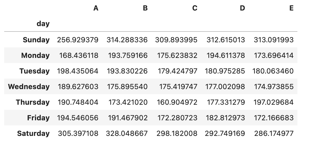
2-3 요일별 각 유형의 평균 전력 사용량 간에 연관성이 있는지 검정하라
- 귀무가설 : 두 변수는 독립적이다
- 대립가설 : 두 변수는 독립적이지 않다.
from scipy.stats import chi2_contingency

chi2, p, dof, expected = chi2_contingency(daydf)
print(p)

# 0.6422684883014576
p-value값이 0.05보다 크기 때문에 귀무가설을 채택한다.
즉, 두 변수는 독립적이라고 할 수있다.
2-4 일자(매일)마다 각 유형의 전력사용량의 합을 데이터프레임으로 구하고 일자 데이터에서의 유형별 온도와의 상관계수를 각각 구하여라
days = q.groupby(q.time.dt.date).sum().reset_index().rename(columns={'time':'date'})
days['date'] = pd.to_datetime(days['date'])

t = pd.read_csv('/kaggle/input/adp-kr-p4/problem2_avg_tem.csv')
t['date'] = pd.to_datetime(t['date'])


pd.merge(t, days).corr().iloc[0,1:].to_frame()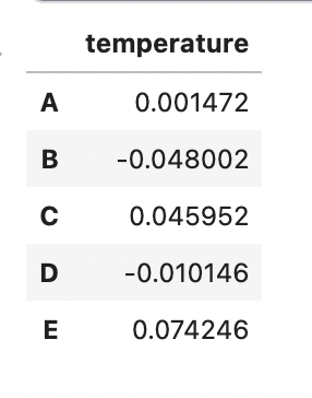
유의미한 상관계수를 가지는 변수는 없음
'adp 실기 > 기출문제' 카테고리의 다른 글
| [Python] 데이터 에듀 ADP 실기 모의고사 4회 3번 파이썬 ver. (비정형 데이터마이닝) (0) | 2022.09.12 |
|---|---|
| [Python] 데이터 에듀 ADP 실기 모의고사 4회 2번 파이썬 ver. (통계분석) (0) | 2022.09.10 |
| [Python] 데이터 에듀 ADP 실기 모의고사 파이썬 ver. (정형 데이터마이닝) (0) | 2022.09.08 |
| [Python] 데이터 에듀 ADP 실기 모의고사 3회 3번 파이썬 ver. (비정형 데이터마이닝) (0) | 2022.09.07 |
| [Python] 데이터 에듀 ADP 실기 모의고사 3회 2번 파이썬 ver. (정형데이터마이닝) (0) | 2022.09.06 |


